
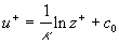
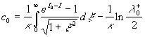
Chaos and Correlation
International Journal, No 5, March 27, 2007
Correlation of Roughness Density Effect on the Turbulent Flow Friction Parameter
By A. P. TRUNEV
The roughness density effect on the mean velocity profile is estimated in the case of 2D and 3D roughness elements. The general correlation for the rough surface friction parameter is proposed.
_____________________________________________________________________
- Introduction
The study of the rough wall turbulence is important in fluid mechanics, in the atmosphere and ocean and in engineering flows. The rough surface effect on the turbulent boundary layer has been considered by Nikuradse (1933) Schlichting (1936, 1960), Bettermann (1966), Dvorak (1969), Simpson (1973), Dirling (1973), Dalle Donne & Meyer (1977), Jackson (1981), Osaka & Mochizuki (1989), Raupach (1992) and other.
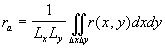
Nikuradse (1933) established (for sand-roughened pipes), that if the roughness height significantly exceeds the viscous sublayer thickness, then the mean velocity profile can be described by the logarithmic function:
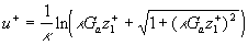
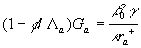
 (1) (1)
where  is the friction velocity, is the friction velocity,  , ,  is the wall shear stress, is the wall shear stress,  is the fluid density, z is the distance from the wall - see Figure 1, is the fluid density, z is the distance from the wall - see Figure 1,  is the characteristic scale of the sand roughness, is the characteristic scale of the sand roughness,  are empirical values. Nikuradse found that are empirical values. Nikuradse found that  for the completely rough regime. He compared the mean velocity profile (1) with the law of the wall, derived by him before in 1932 for turbulent flows in smooth pipes, as follows for the completely rough regime. He compared the mean velocity profile (1) with the law of the wall, derived by him before in 1932 for turbulent flows in smooth pipes, as follows
 (2) (2)
where  is the kinematic viscosity, is the kinematic viscosity,  are the logarithmic profile constants for the hydraulically smooth surface. are the logarithmic profile constants for the hydraulically smooth surface.  is the shift of the mean velocity logarithmic profile which can be defined for the turbulent boundary layer over a rough surface as is the shift of the mean velocity logarithmic profile which can be defined for the turbulent boundary layer over a rough surface as
 (3) (3)
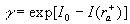
where  for the completely rough regime. Nikuradse has shown that the dimensionless roughness height parameter for the completely rough regime. Nikuradse has shown that the dimensionless roughness height parameter  can be used as an indicator of the rough wall turbulence regime. He proposed to consider three typical cases: can be used as an indicator of the rough wall turbulence regime. He proposed to consider three typical cases:
Thus, the sand-roughened wall turbulence depends on the dimensionless roughness height (roughness Reynolds number)  as has been established by Nikuradse. as has been established by Nikuradse.
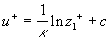
Schlichting (1936), used the Nikuradze's date base and his own experimental results obtained in the water tunnel of rectangular cross section with the upper rough wall, proposed the new form of the equation (1) which is well counted the roughness effect on the turbulent boundary layer by means of the effective wall location ( ) and the equivalent sand roughness parameter ) and the equivalent sand roughness parameter  . With this parameters the mean velocity profile in the turbulent flow over an arbitrary rough surface can be written in the Nikuradze's form (1) as follows: . With this parameters the mean velocity profile in the turbulent flow over an arbitrary rough surface can be written in the Nikuradze's form (1) as follows:
 (4) (4)
where  (see Figure 1). The effective wall location was defined by Schlichting as the mean height of the roughness elements (the location of a "smooth wall that replaces the rough wall in such a manner as to keep the fluid volume the same"). The value has been measured by Schlichting for several types of the roughness elements with various shapes, sizes and spacing. The Schlichting's experiment was re-evaluated by Coleman et. al. (1984) and they noticed that some Schlichting's data have been obtained in the transitional rough regime. (see Figure 1). The effective wall location was defined by Schlichting as the mean height of the roughness elements (the location of a "smooth wall that replaces the rough wall in such a manner as to keep the fluid volume the same"). The value has been measured by Schlichting for several types of the roughness elements with various shapes, sizes and spacing. The Schlichting's experiment was re-evaluated by Coleman et. al. (1984) and they noticed that some Schlichting's data have been obtained in the transitional rough regime.
Clauser (1956) has shown that the shift of the mean velocity profile can be written as

where  is the characteristic scale of roughness elements and is the characteristic scale of roughness elements and  must be some function of the roughness geometrical parameters. Hence the equivalent sand roughness parameter must be some function of the roughness geometrical parameters. Hence the equivalent sand roughness parameter  , where for sand roughness. , where for sand roughness.
Bettermann (1966) discovered that is the function of the roughness elements spacing. He introduced the roughness density parameter for roughness composed of the transverse square bars as the pith-to-height ratio,  - see Figure 1. Bettermann found that in the range - see Figure 1. Bettermann found that in the range  the variations of with the roughness density can be specified by the variations of with the roughness density can be specified by
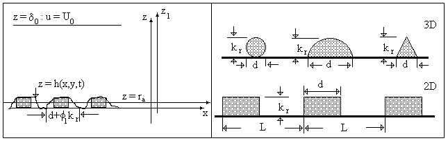
Figure 1: The scheme of the turbulent flow over a rough surface (left), and the roughness elements are considered in the paper (right): spheres, spherical segments, conical elements (3D) and transverse rectangular roods (2D)
As has been demonstrated by Dvorak (1969), the rough wall effect is well correlated with the roughness density parameter defined as pitch-to-width ratio or the ratio of total surface area to roughness area,  . Dvorak developed the Bettermann's model in the range . Dvorak developed the Bettermann's model in the range  , used the data of Schlichting and other researches, as follows: , used the data of Schlichting and other researches, as follows:
 (5) (5)
Simpson (1973) introduced the roughness density parameter in the case of three-dimensional (3D) roughness as  , where , where  is the number of significant roughness elements per unit area, is the number of significant roughness elements per unit area,  is the average frontal area of the "significant" roughness elements. He suggested the general interpretation of the Bettermann-Dvorak correlation (5): two branches (5) exist depending on the formation or absence of transverse vortices between roughness elements. Simpson also showed that the shape of the element is an important parameter. is the average frontal area of the "significant" roughness elements. He suggested the general interpretation of the Bettermann-Dvorak correlation (5): two branches (5) exist depending on the formation or absence of transverse vortices between roughness elements. Simpson also showed that the shape of the element is an important parameter.
The model been reported by Dirling (1973) and verified by Grabow & White (1975), takes into consideration the roughness elements shape parameters. The Dirling's density parameter is defined as  where where  is "the windward wetted surface area". In a case of two-dimensional (2D) roughness the Dirling's parameter leads to the Bettermann's roughness density parameter. As it was shown by Sigal & Danberg (1990) the shape parameters effect can be described by the similar correlation such equation (5) and that is "the windward wetted surface area". In a case of two-dimensional (2D) roughness the Dirling's parameter leads to the Bettermann's roughness density parameter. As it was shown by Sigal & Danberg (1990) the shape parameters effect can be described by the similar correlation such equation (5) and that  for the two-dimensional roughness in the range for the two-dimensional roughness in the range  . They also underlined that the correlation for 2D roughness elements is not the same as for 3D elements. On the other hand, Kind & Lawrysyn (1992) confirmed that the Bettermann-Dvorak function . They also underlined that the correlation for 2D roughness elements is not the same as for 3D elements. On the other hand, Kind & Lawrysyn (1992) confirmed that the Bettermann-Dvorak function  in the form (5) could be successfully used for the correlation of the experimental data in the aerodynamic experiments with the natural hoar-frost roughness. in the form (5) could be successfully used for the correlation of the experimental data in the aerodynamic experiments with the natural hoar-frost roughness.
Dalle Donne & Meyer (1977) correlated their data and those of previous researches used the roughness density parameter  . They developed the empirical model, which can be applied to the turbulent flows in the annuli and tubes with inner surface roughened by rectangular ribs. . They developed the empirical model, which can be applied to the turbulent flows in the annuli and tubes with inner surface roughened by rectangular ribs.
Osaka & Mochizuki (1989) examined d-type rough wall boundary layer in a transitional and a fully rough regime. They have shown that in a transitional rough regime the mean velocity logarithmic profile is confirmed and that the Karman constant has the same value as for the hydraulically smooth wall flow.
The mean velocity logarithmic profile widely used in the atmospheric turbulence research is given by (see Monin & Yaglom (1965)):
where  is the displacement height, is the displacement height,  is the roughness length. Note that and are considered often as some adjustment parameters chosen for the best correlation of the local wind profile in the neutral stratified flow with the logarithmic profile. Jackson (1981) considered the model of the displacement height. Raupach (1992) and other developed the roughness length model. Wieringa (1992) proposed the classification of the experimentally determined roughness length for various terrain types. is the roughness length. Note that and are considered often as some adjustment parameters chosen for the best correlation of the local wind profile in the neutral stratified flow with the logarithmic profile. Jackson (1981) considered the model of the displacement height. Raupach (1992) and other developed the roughness length model. Wieringa (1992) proposed the classification of the experimentally determined roughness length for various terrain types.
The objective of the present work is to develop the model of the turbulent boundary layer which can be applied to any cases considered above: turbulent flows over smooth surfaces, in the transitional rough regime and for the fully developed roughness. The main idea is to derive the model of the turbulent flow over a rough surface directly from the Navier-Stokes equation. As shown in section 2 the requisite model can be derived from the transformed and averaged Navier-Stokes equation due to the surface layer transformation introduced by Trunev & Fomin (1985) in the impingement erosion model and developed by Trunev (1995, 1996, 1997, 1999) for the turbulent boundary layer problem.
2. Turbulent flow model
2.1. Surface layer transformation
The effective wall location was defined by Schlichting (1936) as the mean height of the roughness elements and in the mathematical form can be written as:
 (6) (6)
where  is the relief of the rough surface - see Figure 1, is the relief of the rough surface - see Figure 1,  are the rough wall scales in the are the rough wall scales in the  directions, directions, . In a case of two-dimensional roughness considered by Dvorak (1969) and Simpson (1973) the roughness density parameter depends on width and pitch of the roughness elements (see Figure 1): . The mean roughness height depends on the height of roughness elements as . In a case of two-dimensional roughness considered by Dvorak (1969) and Simpson (1973) the roughness density parameter depends on width and pitch of the roughness elements (see Figure 1): . The mean roughness height depends on the height of roughness elements as  , where , where  is the numerical constant which equals to unity in this case. The shift of the mean velocity can be presented as a function of the mean roughness height. Thus using the Bettermann-Dvorak's equation (5) in the range , we have is the numerical constant which equals to unity in this case. The shift of the mean velocity can be presented as a function of the mean roughness height. Thus using the Bettermann-Dvorak's equation (5) in the range , we have
 = =
In this approach the mean velocity profile in the turbulent flow over a rough surface can be rewritten as follows
If we redefined the main roughness scale then the mean velocity profile takes the form which is widely used in the atmosphere research:
 (7) (7)
where  . Practically . Practically  for for  and and  for for  . Hence, the logarithmic profile mainly depends on the mean height of the roughness elements in this range of the roughness density. . Hence, the logarithmic profile mainly depends on the mean height of the roughness elements in this range of the roughness density.
Let us consider the random function defined as
 (8) (8)
where  is the random parameter with the mean value given by is the random parameter with the mean value given by
here  is the density of a probability distribution function (roughness statistic function) normalised on unity: is the density of a probability distribution function (roughness statistic function) normalised on unity:

Both parts of the equation (8) can be averaged with this function as follows:
where  . With this result the mean-squared-value of the velocity fluctuations can be calculated as . With this result the mean-squared-value of the velocity fluctuations can be calculated as
Thus, the random function  can be used for the mean velocity calculation as well as for the mean-squared-value of the velocity fluctuations modelling. Our main idea is that the random function can be calculated on the basis of some solution of the Navier-Stokes equation due to the surface layer transformation can be used for the mean velocity calculation as well as for the mean-squared-value of the velocity fluctuations modelling. Our main idea is that the random function can be calculated on the basis of some solution of the Navier-Stokes equation due to the surface layer transformation
 (9) (9)
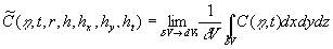
where  is fixed over the integrated region, is fixed over the integrated region,  , ,  is an arbitrary volume put in is an arbitrary volume put in  and containing and containing  as a whole, is the subregion in which altitude of the rough surface as a whole, is the subregion in which altitude of the rough surface  varies in limits from varies in limits from  up to up to  , hence by definition , hence by definition  . .
Note, that the surface layer transformation is only a kind of averaging procedure which conserves the function properties across a boundary layer. The Navier-Stokes equation can be averaged with the surface layer transformation (9) instead of normal Reynolds averaging method to derive then the equation for the random function . Unfortunately it's impossible to use this method in the simple form (9), because, for example, in the case of a smooth flat plate  . .
Therefore we suppose that there is a surface  (the dynamic roughness surface) inside the flow domain which can be used for modelling the rough surface effect on the turbulent boundary layer. Without any limits we can choose a surface close to the wall surface (the dynamic roughness surface) inside the flow domain which can be used for modelling the rough surface effect on the turbulent boundary layer. Without any limits we can choose a surface close to the wall surface  , but not equal to . Let , but not equal to . Let  , where , where  is the height of the viscous sublayer over the rough surface. In the turbulent flow the surface is the height of the viscous sublayer over the rough surface. In the turbulent flow the surface  can be described by random continuous parameters can be described by random continuous parameters  characterising the height, velocity and inclination of the surface elements. Let’s define the subregion in which the local height of the rough surface varies in limits from up to and parameters of the surface in limits from characterising the height, velocity and inclination of the surface elements. Let’s define the subregion in which the local height of the rough surface varies in limits from up to and parameters of the surface in limits from  up to up to  , from , from  up to up to  , from , from  up to up to  , from , from  up to up to  , thus , thus  , where , where  is the multiple density of a probability distribution function. Thus in common case the surface layer transformation can be written as follows (instead of eq. (9)) is the multiple density of a probability distribution function. Thus in common case the surface layer transformation can be written as follows (instead of eq. (9))
 (10) (10)
where  is fixed over the region of integration, is fixed over the region of integration,  , is an arbitrary volume put in and containing as a whole. Statistical moment of an order , is an arbitrary volume put in and containing as a whole. Statistical moment of an order  of a random function of a random function  is given by is given by
 (11) (11)
The main problem of this method is how to estimate the multiple density of a probability distribution function ? Nevertheless, for the solutions presented by the logarithmic function we can suppose that

where the parameters with stars can be estimated from the comparison of solutions with experimental data or calculated from some theoretical considerations. Practically the roughness parameter  should be given as an input value and all another parameters can be calculated from the similarity theory considered in sections 2.6-2.7. should be given as an input value and all another parameters can be calculated from the similarity theory considered in sections 2.6-2.7.
2.2.Input equations
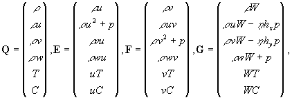
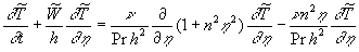
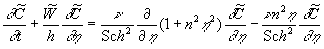
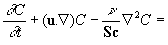
We shall consider the turbulent flow of fluid containing a scalar impurity. Fluid is assumed as viscous, heat-conducting, incompressible gas in a rather slow turbulent motion. Thus, the model of the turbulent flow is given by:
 (12) (12)
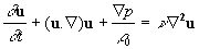
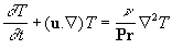 , , 
where is the fluid density,  is the flow velocity vector, is the kinematics viscosity, is the flow velocity vector, is the kinematics viscosity,  is the pressure, is the pressure,  is the temperature, is the temperature,  is the Prandtl number, is the Prandtl number,  is the mass concentration of an impurity, is the mass concentration of an impurity,  is the Schmidt number, is the Schmidt number, is the molecular diffusion coefficient. is the molecular diffusion coefficient.
Boundary conditions for the flow parameters are set as follows:
 (13) (13)

where  is the surface temperature, is the surface temperature,  is the impurity concentration at the wall, is the impurity concentration at the wall,  is the boundary layer thickness, is the boundary layer thickness,  , , are the flow velocity the temperature and the impurity concentration in the distance are the flow velocity the temperature and the impurity concentration in the distance  respectively. respectively.
2.3.Random flow parameters equations
The nontrivial solutions of the Navier-Stokes equations which may play important role in the surface layer turbulent flow organisation can be written as  , where , where  is the dynamic roughness surface. Due to the special type of transformation in the form (10) the velocity field, the pressure, the temperature and concentration are transformed as is the dynamic roughness surface. Due to the special type of transformation in the form (10) the velocity field, the pressure, the temperature and concentration are transformed as
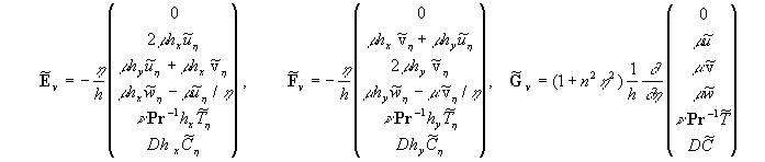
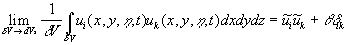
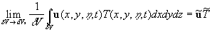
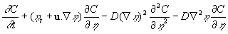
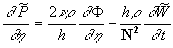
The equations for the random functions  can be derived from the equations (12) written in the curvilinear coordinate system can be derived from the equations (12) written in the curvilinear coordinate system  . Following Pulliam & Steger (1980) the equations (12) are presented in the form: . Following Pulliam & Steger (1980) the equations (12) are presented in the form:
 (14) (14)
where  is the Jacobian, is the Jacobian,  , ,
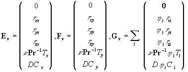
Here  is the tensor of viscous stress, is the tensor of viscous stress,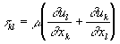 , ,  is the dynamic viscosity, is the dynamic viscosity,  ; ; 
In curvilinear coordinate system it is necessary to execute replacements in terms with gradients:
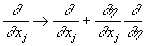 for for  ; ;  , ,
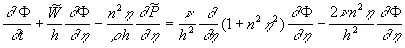
Let us consider the special types of solution of transformed equations (14) which depend only on time and normal variable  as it often suggested in the turbulent boundary layer theory. Thus let’s suppose that as it often suggested in the turbulent boundary layer theory. Thus let’s suppose that  in the left part of (14). In this case eq. (14) can be presented in the form in the left part of (14). In this case eq. (14) can be presented in the form
  (14') (14')
where parameters with tilde are defined similar to  as it follows from (10). In the equation (14') the dissipate terms can be written as as it follows from (10). In the equation (14') the dissipate terms can be written as
where  , .… , .…
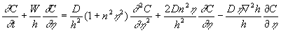
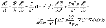
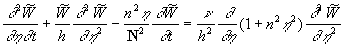
On the other hand to derive the equation (14') one can applied the averaging operator in the form (10) with an arbitrary averaging volume to equation (14) to conserve the commutative properties of the averaging operator with the space and time differential operators. Then one can consider the limit of all terms of the averaged equation at  . At this step the theorem about two limits of the continuous function can be used (since the differential operators can be considered as some limits). Note, if is the solution of the transformed Navier-Stokes equations (14) in any sense, then we have the turbulence model closures automatically as follows: . At this step the theorem about two limits of the continuous function can be used (since the differential operators can be considered as some limits). Note, if is the solution of the transformed Navier-Stokes equations (14) in any sense, then we have the turbulence model closures automatically as follows:
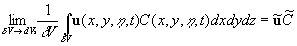
Here  is the kinetic energy of turbulent fluctuations in the small volume is the kinetic energy of turbulent fluctuations in the small volume  , , is the Kronecker delta: is the Kronecker delta:  for for  , ,  for for  . .
Note, that in this model the Reynolds stress can be calculated as

Therefore the random function  gives the main contribution in the non-diagonal components of the Reynolds stress. Now we take it as granted because we haven't any contradictions. Hence, the first assumption of this theory is that the turbulence interaction between the hydrodynamic fields can be described with the solutions as well as with the solutions gives the main contribution in the non-diagonal components of the Reynolds stress. Now we take it as granted because we haven't any contradictions. Hence, the first assumption of this theory is that the turbulence interaction between the hydrodynamic fields can be described with the solutions as well as with the solutions  . The second assumption is that it's possible to neglect longitudinal and transversal gradients of flow parameters in a comparison with gradients across a boundary layer, at least for steady turbulent flow. Finally we have the dynamic equations for random flow parameters as follows: . The second assumption is that it's possible to neglect longitudinal and transversal gradients of flow parameters in a comparison with gradients across a boundary layer, at least for steady turbulent flow. Finally we have the dynamic equations for random flow parameters as follows:
 (15) (15)
where  , ,  , ,  (thus the value (thus the value  included in the turbulent pressure). included in the turbulent pressure).
The first equation (15) is the continuity equation, the second is the momentum equation.
Note, that the parameters of a dynamic roughness in equations (15), are not already the functions of space variables or time. Really, in virtue of transformation (10), the values of these parameters are fixed in intervals from  up to up to , from up to, from up to , fromup to, fromup to. These values, thus, are considered as the random parameters, and the law of their distribution in specific intervals is described by a known function , from up to, from up to , fromup to, fromup to. These values, thus, are considered as the random parameters, and the law of their distribution in specific intervals is described by a known function  . .
As we can see from the derived equations (15) there are the factors in the higher derivatives terms, which depend on a distance up to a rigid surface. It should be noted also, that the equation (14) is not in the strong conservation form, as, for example, it is given by Pulliam & Steger [59]. Therefore the number of terms in a square brackets, breaking conservation of this system are chosen in the left part of equations (14) and (14'). Such allocation of non-divergent terms is stipulated by the purposes of modelling of the eddy viscosity, which, in our opinion, arises in a boundary layer from transformation of a tensor of viscous stresses in a neighbourhood of a dynamic roughness surface. It is obvious in the case of viscous flow over a rigid rough surface and is connected with an adhesion of a viscous flow to a rigid surface of any configuration. In the turbulent flow over a smooth surface the eddy viscosity is simulated by analogy to a more widespread type of turbulent flows, as in a special case, when  . Thus the eddy viscosity is connected (mathematically) with transformation of a tensor of viscous stresses to coordinate mapping which brings rigid surface onto coordinate surface. . Thus the eddy viscosity is connected (mathematically) with transformation of a tensor of viscous stresses to coordinate mapping which brings rigid surface onto coordinate surface.
For the diffusion equation it is possible to derive the boundary layer model by the simplified way. Let us suppose that in the last equation (12) 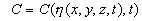 , then we have , then we have
  =0 =0
In partial case when  thus thus
 , ,
and therefore the last equation can be written as
This equation can be transformed to the form of the last equation (15). According to definition
 , ,
Using the identity  , and averaging all terms, finally we have , and averaging all terms, finally we have
where  . But the last term is annulled if region is large enough (the divergence theorem). Therefore we have an equation . But the last term is annulled if region is large enough (the divergence theorem). Therefore we have an equation
  , ,
which is identical to the last equation (15).
2.4. Pressure integral and random flow parameters equations transformation
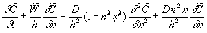
In the case of an isothermal incompressible flow the hydrodynamic part of the equations (15) can be written as:
 (15') (15')
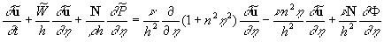
Put  . Multiplying by a scalar way the second equation (15') on the vectors . Multiplying by a scalar way the second equation (15') on the vectors  respectively one can derived the pressure gradient and the equation for the linear combination of momentum components respectively one can derived the pressure gradient and the equation for the linear combination of momentum components  as as
 (16) (16)
where  . Substituting from the continuity equation (15') into the second equation (16) and using the first equation (16) finally we have the closed nonlinear model: . Substituting from the continuity equation (15') into the second equation (16) and using the first equation (16) finally we have the closed nonlinear model:
 (17) (17)
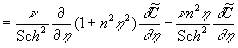
Multiplying the momentum equation (15') on the vector 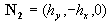 one can derived the linear equation: one can derived the linear equation:
 (18) (18)
where  . .
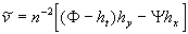
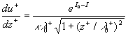
Note, that  is the contravariant component of the velocity vector associated with the vertical turbulent movement. As it follows from (17-18), is the main parameter in this model describing the non-linear turbulent effect. is the contravariant component of the velocity vector associated with the vertical turbulent movement. As it follows from (17-18), is the main parameter in this model describing the non-linear turbulent effect.
2.5.Steady turbulent flow model
In the case of a steady turbulent flow put  in (16-18) then the pressure gradient across boundary layer can be written as in (16-18) then the pressure gradient across boundary layer can be written as
Having substituted this expression in the second equation (16) and rewritten (17-18) in the case of a steady turbulent flow one can find
 (19) (19)
The first integrals of the equations (19) are given by
 , ,  , ,  , (20) , (20)
where  are some constants, are some constants, 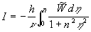 . .
Note, that the velocity components are determined as
 , ,  , , 
hence, used (20) one can derive the velocity gradients equations system written in the normal form suitable for the numerical integration:
 , (21) , (21)
 , , 
2.6. Nonlinear model numerical solution
The first equation (19) has been numerically solved only in the case of the turbulent steady flow over a smooth surface with boundary conditions at
  , (22) , (22)
where  is some free parameter required to obtain the limited value of the integral is some free parameter required to obtain the limited value of the integral  for for  . This condition was used only to obtain the logarithmic asymptotic of the mean velocity. The physical sense of the parameter . This condition was used only to obtain the logarithmic asymptotic of the mean velocity. The physical sense of the parameter  is a clear, because this parameter is direct proportionality to the normal pressure gradient on the wall: is a clear, because this parameter is direct proportionality to the normal pressure gradient on the wall:
, thus  . .
First and second boundary conditions (22) are following from the definition of .
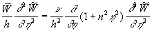
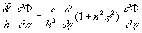
To minimise the number of the independent random parameters the general solution of the first equation (19) can be written as  , where the universal function , where the universal function  depends on the composition of random parameters (the dynamic roughness Reynolds number): depends on the composition of random parameters (the dynamic roughness Reynolds number):
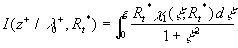
 (23) (23)
and satisfies to the equation
 (24) (24)
with boundary conditions at
  (25) (25)
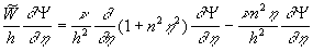
where , ,  is also the free parameter required to obtain the limited value of the integral is also the free parameter required to obtain the limited value of the integral  at at  . Note, that (24) can be easily derived from the first equation (19). Consequently the integral depends on the composition of random parameters . Note, that (24) can be easily derived from the first equation (19). Consequently the integral depends on the composition of random parameters  and can be calculated as and can be calculated as
 (26) (26)
The integral (26) has been computed in the range  together with (24-25). Fourth-order scaled Runge-Kutta algorithms and the shooting method have been used to get the numerical solution. Note that for together with (24-25). Fourth-order scaled Runge-Kutta algorithms and the shooting method have been used to get the numerical solution. Note that for  this problem has the analytical solution: this problem has the analytical solution:
 . .
In this case  , hence one can suggested that function , hence one can suggested that function
has a limited value at . It is possible if only  , thus , thus
This solution has been used as the initial position in the shooting method.
The normalized function  is shown in Figure 2,a for the various is shown in Figure 2,a for the various  - the solid lines 1-5 respectively. As well seen is a simple and smooth function such - the solid lines 1-5 respectively. As well seen is a simple and smooth function such  . .
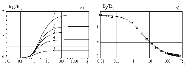
Figure 2: a) The normalised function computed on equations (24, 26) for the various  - the solid lines 1-5 respectively; b) The normalised integral - the solid lines 1-5 respectively; b) The normalised integral  versus the dynamic roughness parameter calculated for versus the dynamic roughness parameter calculated for 
The calculated limited value  is shown in Figure 2,b by the symbols together with the approximated line is shown in Figure 2,b by the symbols together with the approximated line
 (27) (27)
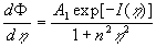
To simplifier the numerical modelling of the mean velocity profile over a rough surface the function  has been approximated as has been approximated as
 (28) (28)
where  is given by (27). is given by (27).
Finally note, that for the negative value of the parameter  in the range in the range  the numerical procedure becomes unstable one. In this case the value much increases with the small decreasing of the dynamic roughness parameter . Since this branch of the integral will not be used in the our analysis, therefore data for the negative value the numerical procedure becomes unstable one. In this case the value much increases with the small decreasing of the dynamic roughness parameter . Since this branch of the integral will not be used in the our analysis, therefore data for the negative value  is not presented in Figure 2, b and has been neglected in approximation formula (27). is not presented in Figure 2, b and has been neglected in approximation formula (27).
2.7. Mean velocity logarithmic profile in turbulent flow over smooth surface
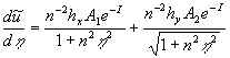
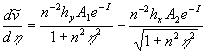
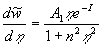
The turbulent boundary layer over a smooth surface is the best example for the theoretical consideration and modelling with the model (21). In this case the streamwise velocity gradient can be written in the standard form used the inner layer variables  , ,  , and boundary conditions for the mean velocity gradient: , and boundary conditions for the mean velocity gradient:
at  ; ;
at  , ,
where  is the Karman constant. As it was suggested in subsection 2.1 we have used parameters with stars instead of random parameters. Finally we have for the streamwise velocity gradient is the Karman constant. As it was suggested in subsection 2.1 we have used parameters with stars instead of random parameters. Finally we have for the streamwise velocity gradient
 (29) (29)
where  , ,  . .
The first term in the right part (29) has the essential value mainly close to the wall and the second one gives the main contribution in the logarithmic layer. To derive the mean velocity profile we should defined firstly the parameter . Note, from first equation (21) and (29) it follows that
where  , ,  . Our suggestion about the dynamical roughness structure is that the parameter fluctuates around the mean value . Our suggestion about the dynamical roughness structure is that the parameter fluctuates around the mean value  . This structure looks like furrows elongated along of the mean flow stream lines in the viscous sublayer (see, for instance, Cantwell, Coles & Dimotakis (1978) where some visualization of the coherent structure in the turbulent boundary layer is presented). . This structure looks like furrows elongated along of the mean flow stream lines in the viscous sublayer (see, for instance, Cantwell, Coles & Dimotakis (1978) where some visualization of the coherent structure in the turbulent boundary layer is presented).
Thus for the mean flow  , then the length scale can be found as the solution of the equation , then the length scale can be found as the solution of the equation
 (30) (30)
where  , ,  is the second scale of the turbulent velocity. For an arbitrary value is the second scale of the turbulent velocity. For an arbitrary value  the equation (30) has two roots or hasn't any roots and only if the equation (30) has two roots or hasn't any roots and only if  this equation has one root. Hence for the uniqueness of the mean velocity profile should be this equation has one root. Hence for the uniqueness of the mean velocity profile should be
 (31) (31)
The numerical solution of the equation (31) with determined from (27) gives  and therefore the predicted values of the turbulent theory constants are given by and therefore the predicted values of the turbulent theory constants are given by  , ,  for for  . The fundamental parameter of length for the turbulent boundary layer is defined from here: . The fundamental parameter of length for the turbulent boundary layer is defined from here:  , that almost coincides with the peak of turbulence production , that almost coincides with the peak of turbulence production  , obtained by Klebanoff (1954) and Laufer (1954) - see for instance Rotta (1972) (this book has been kindly indicated by referee). , obtained by Klebanoff (1954) and Laufer (1954) - see for instance Rotta (1972) (this book has been kindly indicated by referee).
If  then then  in (29) and this equation can be presented in the form: in (29) and this equation can be presented in the form:
 , ,  (32) (32)
Integrated the first equation (32) we have:
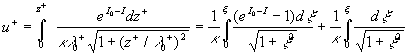 = =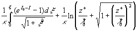
The standard logarithmic profile can be derived from here at  : :
 , ,  . (33) . (33)
Therefore, with the given constant  another constant of the mean velocity logarithmic profile can be calculated from (33). It gives another constant of the mean velocity logarithmic profile can be calculated from (33). It gives  for for  . .
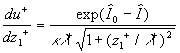
The velocity profile calculated with (32) for 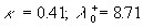 is shown in Figure 3,a - the solid line (1). The predicted profile (1) has been compared with the mean velocity computed on the model of the transitional layer proposed by Van Driest (1956) - the solid line (2). As explained by Cebeci & Bradshaw (1984) the Van Driest's model can be written in the form is shown in Figure 3,a - the solid line (1). The predicted profile (1) has been compared with the mean velocity computed on the model of the transitional layer proposed by Van Driest (1956) - the solid line (2). As explained by Cebeci & Bradshaw (1984) the Van Driest's model can be written in the form
 , ,  (34) (34)
where  is the damping length, is the damping length,  . .
The profile computed on (34) coincides with the predicted profile 1 in the viscous sublayer and in the logarithmic layer but smaller differs in the transitional layer (see Figure 3, a). This difference can be explained by the pressure gradient effects. Figure 3,b demonstrates the comparison of both profiles (1,2) with the several data bases: 3 - the direct numerical simulation of the turbulent flow in the two-dimensional channel ( ) by Kuroda et al (1989); 4 - the turbulent boundary layer in zero pressure gradient ( ) by Kuroda et al (1989); 4 - the turbulent boundary layer in zero pressure gradient ( ) by Nagano et al (1992) and 5 - the turbulent boundary layer mean velocity profile ( ) by Nagano et al (1992) and 5 - the turbulent boundary layer mean velocity profile ( ) presented by Smith (1994). As can seen both profiles well correlated with computed and experimental data. ) presented by Smith (1994). As can seen both profiles well correlated with computed and experimental data.
In the upper layer for  the mean velocity profile should be constant in contrast to the logarithmic profile which diverges at the mean velocity profile should be constant in contrast to the logarithmic profile which diverges at  . As well known in the outer region of the turbulent boundary layer the mean velocity profile can be described by the defect low . As well known in the outer region of the turbulent boundary layer the mean velocity profile can be described by the defect low  , where the universal function , where the universal function  is weakly dependent on the Reynolds number and roughness parameters in the case of a zero pressure gradient. is weakly dependent on the Reynolds number and roughness parameters in the case of a zero pressure gradient.
One can suggested, that the mixed layer turbulence is generated by the same way like the wall turbulence. Then the new dynamic roughness surface can be introduced and the equation system which is similar to (21) can be derived. In the case of the mixing layer we can put  . With two characteristic scales . With two characteristic scales  and and  the general solution for the boundary layer mean velocity profile can be written as (see Trunev (1999)) the general solution for the boundary layer mean velocity profile can be written as (see Trunev (1999))
 (35) (35)
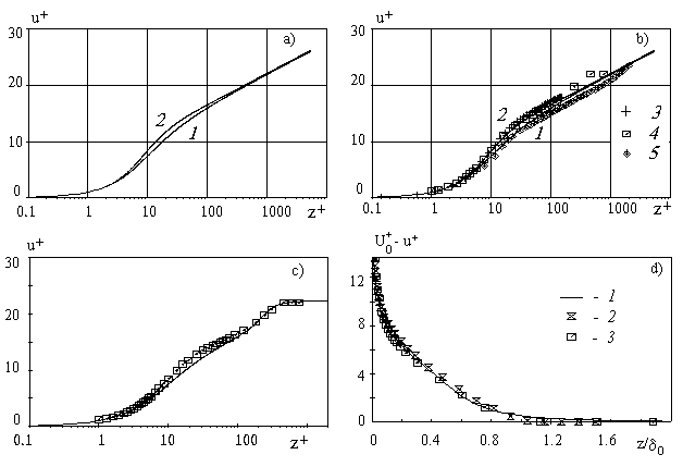
Figure 3. Mean velocity profile in the turbulent boundary layer: a) profiles computed on the present model (1) and van Driest model (2); b) comparison of computed profiles (1-2) with DNS data (3) and experimental data (4-5); c) the solid line is computed on eq.(35), experimental data Nagano et all (1992) presented by symbols d) defect low: the solid line 1 is computed on eq. (35), 2,3 - experimental data by Nagano et all (1992)
where  , ,  is the middle position of the mixing layer, is the middle position of the mixing layer,  , ,  is the mean velocity profile in the inner layer given by eq. (32), is the mean velocity profile in the inner layer given by eq. (32),  . .
Profile (35) depends on two dimensionless values which have been defined from experimental data as  . The mean velocity profile and defect low calculated on (35) are shown in Figure 3, c-d, together with experimental data by Nagano et all (1992). As can seen from this data the agreement between theoretical and experimental results in general is good. . The mean velocity profile and defect low calculated on (35) are shown in Figure 3, c-d, together with experimental data by Nagano et all (1992). As can seen from this data the agreement between theoretical and experimental results in general is good.
3. Rough surface effects modelling
3.1. Rough surface model
The additive dynamic roughness surface model considered above is given by
where is the height of the viscous sublayer over the rough surface. Averaged this equation over a large area one can derived: 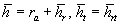 , where , where  is the mean roughness height: is the mean roughness height:
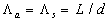
After replacing of the origin of the coordinate system in the new position  the dynamic roughness equation can be written as: the dynamic roughness equation can be written as:
 (36) (36)
where 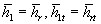 . Thus, we can imagine the smooth wall located at . Thus, we can imagine the smooth wall located at  as was defined by Schlichting (1936) and the dynamic roughness surface with dynamic roughness parameters given by (36). For this problem we should suggest that as was defined by Schlichting (1936) and the dynamic roughness surface with dynamic roughness parameters given by (36). For this problem we should suggest that  . .
Note that the fluid flow nearly the plate is a typical heterogeneous flow included two parts: the roughness rigid elements part  and the fluid flow part equal to and the fluid flow part equal to  , where , where  . Put . Put 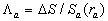 is the ratio of the whole area to the roughness area at . The roughness density parameter proposed by Dvorak (1969) is given by is the ratio of the whole area to the roughness area at . The roughness density parameter proposed by Dvorak (1969) is given by  , where S is the total roughness area. Since , where S is the total roughness area. Since  , thus , thus  can be considered as a function of the Dvorak's roughness parameter: can be considered as a function of the Dvorak's roughness parameter:  . For the roughness elements considered by Bettermann (1966), Schlichting (1936) and Coleman et. al. (1984) this function can be calculated in the closure form. . For the roughness elements considered by Bettermann (1966), Schlichting (1936) and Coleman et. al. (1984) this function can be calculated in the closure form.
For the roughness compounds by the spherical uniform elements  , , 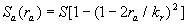 , hence , hence
 (37,a) (37,a)
In the case of the surface rounded by spherical segments (see Figure 1) we have: 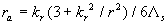 , , 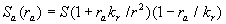 , therefore , therefore
 (37,b) (37,b)
where,  . .
In the case of the surface with conical uniform elements 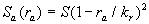 , ,  , thus , thus
 (37,c) (37,c)
In the case of two dimensional roughness such have been considered by Bettermann (1966), Dvorak (1969) and Dalle Donne & Meyer (1976) depends on only the roughness elements width and pitch (see Figure 1):
 (37,d) (37,d)
The mean liquid surface between the roughness elements at equal to , therefore the mean fluid density , therefore the mean fluid density 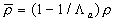 (note that in the real case additionally some liquid volume can be exclude from the mean flow, hence can be (note that in the real case additionally some liquid volume can be exclude from the mean flow, hence can be 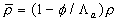 where where  is the shape parameter counted for instance the liquid involved in the viscous sublayer around the roughness elements). The mean dynamic viscosity is defined as is the shape parameter counted for instance the liquid involved in the viscous sublayer around the roughness elements). The mean dynamic viscosity is defined as 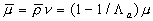 . .
Thus is the important parameter for the rough surface effects modelling because the boundary condition for the mean velocity gradient should be given at .
3.2. Mean velocity logarithmic profile in turbulent flow over rough surface
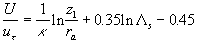
The mean velocity logarithmic profile in the turbulent flow over the rough surface can be derived from (32) written in the new coordinate system:
 , ,  (38) (38)
where  , ,  , ,  , ,  . .
The boundary condition for the equation (38) on the effective smooth wall is given by
 at at  (39, a) (39, a)
where  is the effective shear stress applied to the effective smooth wall at . Thus for the dimensionless mean velocity gradient on the effective wall in common case one can proposed the equation is the effective shear stress applied to the effective smooth wall at . Thus for the dimensionless mean velocity gradient on the effective wall in common case one can proposed the equation
 at (39, b) at (39, b)
As follows from the mean velocity logarithmic profile in the turbulent flow established by Schlichting (see eq. (4)) the dimensionless turbulent length in the first equation (38) depends on the roughness parameters and thus can't be defined from an equation similar to eq. (30). To define  note, that for the completely rough regime in the classical sense, when note, that for the completely rough regime in the classical sense, when  , one can supposed that , one can supposed that  . Then the exact solution of the problem (38-39) can be written as . Then the exact solution of the problem (38-39) can be written as
 (40) (40)
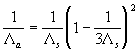
But this equation also follows from (38) if we put  in the non-linear model (24), and therefore in the non-linear model (24), and therefore  . Hence, in the case of turbulent flow over a rough surface the main turbulent length scale can be defined as . Hence, in the case of turbulent flow over a rough surface the main turbulent length scale can be defined as 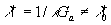 , and the second scale of the turbulent velocity equal zero. , and the second scale of the turbulent velocity equal zero.
The mean velocity logarithmic profile follows from (40) at the long distance from the wall. Put  in (40), then we have in (40), then we have
 , where , where 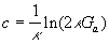 . .
This equation easily can be rewritten in the standard form as follows:
 , ,  (41) (41)
where  . Note, that the finale result (41) mainly depends on the mean velocity gradient applied to the effective smooth surface at . . Note, that the finale result (41) mainly depends on the mean velocity gradient applied to the effective smooth surface at .
3.3. Roughness density effect model
There are two available cases can be realised in the experimental situation: the roughness elements installed on the absolutely smooth surface and the roughness elements installed on the rough surface. In the first case we surmise that the mean velocity gradient applied to the effective smooth wall is proportional to the velocity gradient over a smooth surface given by the first equation (32) for . Used the boundary condition (39,b) we have:
 (42) (42)
where the shape parameter introduced to estimate the frontal and leeward re-circulation zones effects,  , ,  is some parameter. Suggested that is some parameter. Suggested that  where where  is a function of the roughness parameters, we have for the smooth background surface: is a function of the roughness parameters, we have for the smooth background surface:
 , ,  (43) (43)
here  is the transitional layer parameter. Note, that for the high value of the roughness density parameter may be (completely rough regime in the classical sense), but simultaneously is the transitional layer parameter. Note, that for the high value of the roughness density parameter may be (completely rough regime in the classical sense), but simultaneously 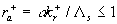 . Thus . Thus  for the completely rough regime in the non-classical sense defined only for for the completely rough regime in the non-classical sense defined only for  as follows from the second equation (43). The main turbulent length scale can be estimated from (43) as as follows from the second equation (43). The main turbulent length scale can be estimated from (43) as 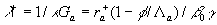 . .
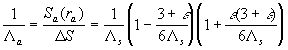
Substituted  from (43) into the second equation (41) finally we have: from (43) into the second equation (41) finally we have:
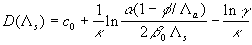 (44) (44)
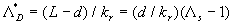
The rough surface effects model (44) depends on two parameters  chosen from the best correlation with the experimental data. We should underlined that chosen from the best correlation with the experimental data. We should underlined that  is the friction parameter of the rough surface and is the friction parameter of the rough surface and  is the parameter of the mean density of fluid involved in the mean turbulent flow at the level . is the parameter of the mean density of fluid involved in the mean turbulent flow at the level .
In the second case the mean velocity gradient model is the same as (44) but we should put  where where  is the averaged height of the background roughness. Both models have been testified and shown the good agreement with the experimental data. is the averaged height of the background roughness. Both models have been testified and shown the good agreement with the experimental data.
3.4. Modelling of roughness density effects. 3D roughness elements
To test the roughness surface effect model (44) the turbulent flow data for 3D roughness elements obtained by Schlichting (1936) and re-evaluated by Coleman et. al. (1984) have been used. The main result reported by Coleman et. al. (1984) is that some Schlichting's data were obtained probably in the transitionally rough regime. The experimental techniques in Schlichting's (1936) and Coleman et. al. (1984) experiments have been analyzed and it was surmised that Schlichting's data were measured in the fully rough regime but some details of his experimental technique have not been reported.
The computed (1) and experimental data by Schlichting (3) and Coleman et. al. (5) are shown in Figure 4 for spheres (Fig. 4,a), spherical segments (Fig. 4,b) and cones (Fig. 4,c). The points (4) are computed from the experimental data by Coleman et. al. (5) which have been corrected with transitional layer parameter calculated on (27-28) as follows  . As can seen the transitional layer effect is essential for the plate with roughness in a form of spherical segments (two points with . As can seen the transitional layer effect is essential for the plate with roughness in a form of spherical segments (two points with  and consequently and consequently  ) and conical elements (two points with ) and conical elements (two points with  and respectively), and relatively small for all data with and respectively), and relatively small for all data with  , included data for the plate roughened by spheres. Note, that the experimental data re-evaluated by Coleman et. al. (1984) become near by to the original Schlichting's data after the correction on the transitional layer effect. Therefore it seems to be clear that the data by Coleman et. al. (1984) is based on the another experimental technique then the original Schlichting's data. , included data for the plate roughened by spheres. Note, that the experimental data re-evaluated by Coleman et. al. (1984) become near by to the original Schlichting's data after the correction on the transitional layer effect. Therefore it seems to be clear that the data by Coleman et. al. (1984) is based on the another experimental technique then the original Schlichting's data.
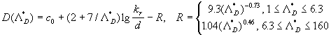
The corrected data have been used to estimate the parameters in the equation (44) which can be written for the completely roughness regime () as follows
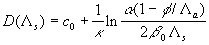 (45) (45)
where the roughness parameters  are given by (37, a-c) for the spheres, spherical segments and conical elements respectively. are given by (37, a-c) for the spheres, spherical segments and conical elements respectively.
As has been established in the case of the plate with spheres  , ,  for the data obtained by Coleman et. al. (1984) (solid line (1) in Figure 4,a) and for the data obtained by Coleman et. al. (1984) (solid line (1) in Figure 4,a) and  , ,  for the corrected points. For the roughness elements in the form of spherical segments for the corrected points. For the roughness elements in the form of spherical segments  , ,  (solid line (1), Figure 4,b) and for the conical elements (solid line (1), Figure 4,b) and for the conical elements  , - see Figure 4,c. For comparison the Bettermann-Dvorak's correlated line (2) also is shown in Figure 4. , - see Figure 4,c. For comparison the Bettermann-Dvorak's correlated line (2) also is shown in Figure 4.
The magnitude  can be explained in terms of the rough surface drag which has the same value for the spheres and conical elements and mach less for the surface with spherical segments. The mean fluid density parameter can be explained in terms of the rough surface drag which has the same value for the spheres and conical elements and mach less for the surface with spherical segments. The mean fluid density parameter  for considered types of roughness elements. Note that in the case of the surface roughened by spheres the function has a maximum at for considered types of roughness elements. Note that in the case of the surface roughened by spheres the function has a maximum at  (as has been established in numerical experiments the maximum location depends on the value approximately as (as has been established in numerical experiments the maximum location depends on the value approximately as  for the range for the range ). ).
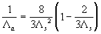
Figure 4. Roughness density effect on the turbulent flow in a case of 3D roughness elements: a) spheres; b) spherical segments; c) cones; d) the generalised correlation
The experimental data for the surfaces with spheres, spherical segments or conical elements can be collected together used some "universal" parameter another one then proposed by Bettermann (Dvorak (1969), Dirling (1973), Simpson (1973), Kind & Lawrysyn (1992) and other. This correlation is available for the high roughness density parameter at  , then , then
and therefor the "universal" parameter is given by  . The solid line (1) computed on the equations (37,a), and (45) for . The solid line (1) computed on the equations (37,a), and (45) for  , is shown in Figure 4, d with the corrected experimental data for the rough surfaces with spheres (2), spherical segments (3) and conical elements (4) . The classic sandgrain-roughened pipe flow experiment of Nikuradse (1933) with , is shown in Figure 4, d with the corrected experimental data for the rough surfaces with spheres (2), spherical segments (3) and conical elements (4) . The classic sandgrain-roughened pipe flow experiment of Nikuradse (1933) with  is presented by point (5). The hoar frost roughness data of Kind & Lawrysyn (1992) are plotted by points (6). Note, that data of Kind & Lawrysyn (1992) have been corrected with transitional layer parameter is presented by point (5). The hoar frost roughness data of Kind & Lawrysyn (1992) are plotted by points (6). Note, that data of Kind & Lawrysyn (1992) have been corrected with transitional layer parameter

where ,  is the averaged height of the background roughness, is the averaged height of the background roughness,  depends on the frost formation and has been calculated for the plate 1-6 of Kind & Lawrysyn (1992) as follows depends on the frost formation and has been calculated for the plate 1-6 of Kind & Lawrysyn (1992) as follows  . In this case as for the conical elements. The experimental data for 3D rounded elements of Simpson (1973) are shown by symbols (7). For his data . In this case as for the conical elements. The experimental data for 3D rounded elements of Simpson (1973) are shown by symbols (7). For his data  . .
Thus one can suggested that the rough surface with spheres is the basic case for 3D roughness elements, because all data shown in the Figure 4, d are correlated well with the basic line (1).
Then one can propose the model for considered this parameter as some function of the width-to-height ratio considered this parameter as some function of the width-to-height ratio 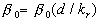 . For instance, at . For instance, at  we have the Dvorak's roughness density parameter we have the Dvorak's roughness density parameter 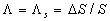 . For a linear function the "universal" parameter is related to that of Bettermann (1966) since in the case of transverse square bars . For a linear function the "universal" parameter is related to that of Bettermann (1966) since in the case of transverse square bars  and hence and hence  , where , where  is some numerical value. is some numerical value.
3.5. Modelling of roughness density effects. 2D roughness elements
The empirical model of Dalle Donne & Meyer (1977) for 2D roughness composed by the transverse rectangular rods is based on the roughness density parameter
With this parameter the experimental data of Dalle Donne & Meyer (1977) and other sources summarized in Table I can be described as follows
 (46) (46)
This correlation has been derived by Dalle Donne & Meyer (1977) for the range of the experimental data parameters 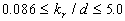 and and  . .
As can seen from (46) the rough surface effect depends on two roughness parameters  and and  . Thus, there is no any "universal" parameter for 2D roughness elements in the common case. But the experimental data with various can be plotted together as the graph of the function . Thus, there is no any "universal" parameter for 2D roughness elements in the common case. But the experimental data with various can be plotted together as the graph of the function  . Figure 5 demonstrates . Figure 5 demonstrates  calculated on ( 46) - solid line (1) and the experimental data found for 2D roughness elements by various authors listed in Table 1 (the corrected and reduced data or calculated on ( 46) - solid line (1) and the experimental data found for 2D roughness elements by various authors listed in Table 1 (the corrected and reduced data or  from Table 2 of Dalle Donne & Meyer (1977) have been used as long as correlation (46) proposed for this values).The symbols description is given in the right part of Figure 5 and Table 1. As can seen the correlation is good for the middle and high value of the roughness density parameter, but for from Table 2 of Dalle Donne & Meyer (1977) have been used as long as correlation (46) proposed for this values).The symbols description is given in the right part of Figure 5 and Table 1. As can seen the correlation is good for the middle and high value of the roughness density parameter, but for  the scatter of the points is rather large and can't be explained by the experimental technique differences only. the scatter of the points is rather large and can't be explained by the experimental technique differences only.
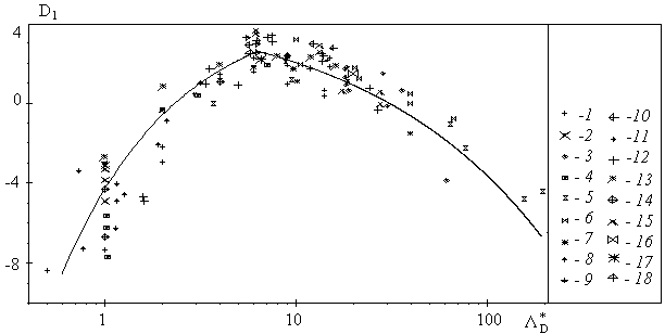
Figure 5:  vs vs  - the solid line. 2D roughness elements data 1-18 have been obtained by authors listed in Table 1 - the solid line. 2D roughness elements data 1-18 have been obtained by authors listed in Table 1
Used the roughness density parameter model in the form (37, d) and suggested that (completely rough regime) one can written (44) for this case as follows
 (47) (47)
For the constant value of the parameters the function has a maximum at  . This maximum can be defined from (46) as . This maximum can be defined from (46) as  , and therefore , and therefore  . Thus as it follows from the experimental data the shape parameter varies with . To compare the experimental data with the arbitrary value of the shape parameter let us introduce the roughness density parameter in the form . Thus as it follows from the experimental data the shape parameter varies with . To compare the experimental data with the arbitrary value of the shape parameter let us introduce the roughness density parameter in the form  , then the roughness density effect model (47) can be rewritten as , then the roughness density effect model (47) can be rewritten as
 (48) (48)
where  . .
Table 1
|
Authors |
Year |
Geometry |

|
|
Symbol |
|
Möbius |
1940 |
Tube |
10.0-29.22 |
0.3-2.20 |
3 |
|
Chu & Streeter |
1949 |
Tube |
1.95-7.57 |
0.93 |
4 |
|
Sams |
1952 |
Tube |
2.0-2.3 |
0.88-1.37 |
9 |
|
Nunner |
1956 |
Tube |
16.36 |
0.8 |
16 |
|
Koch |
1958 |
Tube |
9.8-980 |
1.0-5.0 |
5 |
|
Fedynskii |
1959 |
Annulus |
6.67-16.7 |
1.0 |
10 |
|
Draycott & Lawther |
1961 |
Annulus |
2.0 |
1.0 |
2 |
|
Skupinski |
1961 |
Annulus
Tube |
2.0-41.0
22.2-133.4 |
1.0
2.0 |
6 |
|
Savage & Myers |
1963 |
Tube |
3.66-43.72 |
1.33-2.67 |
13 |
|
Perry & Joubert |
1963 |
Wind tunnel |
4.0 |
1.0 |
19 |
|
Sheriff, Gumley & France |
1963 |
Annulus |
2.0-10.0 |
1.0 |
14 |
|
Gargaud & Paumard |
1964 |
Tube
Annulus |
1.8-16.0
10.0-16.0 |
1.0-1.67
1.0 |
1 |
|
Bettermann |
1966 |
Wind tunnel |
2.65-4.18 |
1.0 |
20 |
|
Massey |
1966 |
Annulus |
7.53-30.15 |
1.06 |
15 |
|
Kjellström & Larson |
1967 |
Annulus |
2.02-38.52 |
0.086-4.08 |
12 |
|
Fuerstein & Rampf |
1969 |
Annulus |
2.91-25.04 |
0.42-2.50 |
8 |
|
Lawn & Hamlin |
1969 |
Annulus |
7.61 |
1.0 |
17 |
|
Watson |
1970 |
Annulus |
6.49-7.22 |
1.0 |
11 |
|
Stephens |
1970 |
Annulus |
7.20 |
1.0 |
18 |
|
Webb, Eckert & Goldstein |
1971 |
Tube |
9.70-77.63 |
0.97-3.88 |
7 |
|
Antonia & Luxton |
1971 |
Wind tunnel |
4.0 |
1.0 |
21 |
|
Antonia & Wood |
1975 |
Wind tunnel |
2.0 |
1.0 |
22 |
|
Dalle Donne & Meyer |
1977 |
Annulus |
4.08-61.5 |
0.25-2.0 |
24 |
|
Pineau, Nguyen, Dickinson & Belanger |
1987 |
Wind tunnel |
4.0 |
1.0 |
23 |
In this model the experimental data for various can be plotted together as the graph of the function  as well as in the Dalle Donne & Meyer's model (46). But as has been established the shape parameter derived from the model (46) isn't the good approximation. as well as in the Dalle Donne & Meyer's model (46). But as has been established the shape parameter derived from the model (46) isn't the good approximation.
Note that in the common case one can suggested that  , where , where  is the total length of the frontal and leeward re-circulation zones. The model (46) gives for this parameter the unphysical result is the total length of the frontal and leeward re-circulation zones. The model (46) gives for this parameter the unphysical result  . Thus the experimental data of various authors listed in Table 1 have been used to find the right form of and . Thus the experimental data of various authors listed in Table 1 have been used to find the right form of and  . The best correlation for about 130 points is given by . The best correlation for about 130 points is given by
 , ,  (49) (49)
where  . .
Figure 6 shows  calculated on (48-49) - the solid line (1), and the experimental data 1-24 of various authors listed in Table 1 (note, we have used values calculated on (48-49) - the solid line (1), and the experimental data 1-24 of various authors listed in Table 1 (note, we have used values  from Table 2 of Dalle Donne & Meyer (1977) instead of the original data 1-18). The symbols description is given in the right part of Figure 6 and in Table 1. Some fragment of the correlated line is shown in the lower part of Figure 6. One can seen that the predicted roughness density effects (solid line) is in a good agreement with the available experimental data. from Table 2 of Dalle Donne & Meyer (1977) instead of the original data 1-18). The symbols description is given in the right part of Figure 6 and in Table 1. Some fragment of the correlated line is shown in the lower part of Figure 6. One can seen that the predicted roughness density effects (solid line) is in a good agreement with the available experimental data.
Finally note, that (49) are derived for the rough surface composed by the transverse rectangular rods and can't be applied to 2D roughness elements of another form without additionally verification.
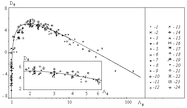
Figure 6:  vs vs  - the solid line. 2D roughness elements data 1-24 have been obtained by authors listed in Table 1 - the solid line. 2D roughness elements data 1-24 have been obtained by authors listed in Table 1
3.6. Model of the total length of the frontal and leeward re-circulation zones
Analyzed expression (48) one can found two singular points:  , and , and  , which correspond to two branches of function . Dalle Donne & Meyer (1977) model (46) also has two singular points , which correspond to two branches of function . Dalle Donne & Meyer (1977) model (46) also has two singular points  and and  . Taken into account that . Taken into account that  one can concluded that this two singular points are approached at one can concluded that this two singular points are approached at  and and  accordingly. As can seen from the data shown in Figures 5 there is probably one singular point more at accordingly. As can seen from the data shown in Figures 5 there is probably one singular point more at  . All data collected around the point at have been obtained mainly for . All data collected around the point at have been obtained mainly for  . Thus this point can be at . Thus this point can be at  . But what the physical reason for this point generally speaking? In Figure 7, a) the normalised total length of the frontal and leeward re-circulation zones (solid lines) dependent on the Dvorak's roughness density parameter . But what the physical reason for this point generally speaking? In Figure 7, a) the normalised total length of the frontal and leeward re-circulation zones (solid lines) dependent on the Dvorak's roughness density parameter  and the mean fluid density (broken line) calculated for and the mean fluid density (broken line) calculated for  are shown. are shown.
Figure 7. à) the normalised total length of the frontal and leeward re-circulation zones (solid lines) dependent on the Dvorak's roughness density parameter and the normalised mean fluid density (broken line) calculated for .
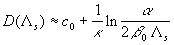
b) the roughness density effect on the mean velocity shift  at fixed at fixed  : the solid lines 1 are calculated on the model (45)-(49), The solid line 2 is calculated on (45)-(49) where : the solid lines 1 are calculated on the model (45)-(49), The solid line 2 is calculated on (45)-(49) where was decreased on 10% was decreased on 10%
As can seen from Figure 7, a) the total length has a maximum located in some point  . Accordingly to this the effective mean fluid density has a minimum which can be less then zero. As it follows from (39, b), if is limited value and . Accordingly to this the effective mean fluid density has a minimum which can be less then zero. As it follows from (39, b), if is limited value and  then then  thus it will be some singular point for the function thus it will be some singular point for the function  . Physically it means that the frontal and leeward re-circulation zones have intersection. As well known in this case the skimming flow is realised. In the present model this regime counted statistically and probably with some error. In any case all data over point in Figure 5 are replaced to the point . Physically it means that the frontal and leeward re-circulation zones have intersection. As well known in this case the skimming flow is realised. In the present model this regime counted statistically and probably with some error. In any case all data over point in Figure 5 are replaced to the point  in Figure 6. Note that correlated line goes throughout these data better in Figure 6 than in Figure 5. in Figure 6. Note that correlated line goes throughout these data better in Figure 6 than in Figure 5.
An unexpected result has been found in numerical experiment that function has one maximum for  and two maximum for and two maximum for  as shown by the solid lines 1 in Figure 7, b calculated for . This result is a very sensitive to the variations of the value . If is multiplied on 0.9 then the function lost the singular point and looks like solid line 2 in Figure 7. Now we have only experimental data shown in Figure 7 which not sufficient to confirm this result. as shown by the solid lines 1 in Figure 7, b calculated for . This result is a very sensitive to the variations of the value . If is multiplied on 0.9 then the function lost the singular point and looks like solid line 2 in Figure 7. Now we have only experimental data shown in Figure 7 which not sufficient to confirm this result.
Some restriction for this model can be established if the length scale  found for the rough surfaces is compared with the main turbulent length scale found for the rough surfaces is compared with the main turbulent length scale  computed for the boundary layer over a smooth surface as computed for the boundary layer over a smooth surface as  . It gives for 2D roughness considered above that the normalised mean fluid density is limited as . It gives for 2D roughness considered above that the normalised mean fluid density is limited as  . If this restriction is broken then it means that the model (48) also can't be used properly. Supposed that in this case . If this restriction is broken then it means that the model (48) also can't be used properly. Supposed that in this case  one can regularised the function in the singular point shown in Figure 7,b. one can regularised the function in the singular point shown in Figure 7,b.
- Conclusion
The turbulent boundary layer model has been derived directly from the Navier-Stokes equations. The model is based on the special type of the Navier-Stokes equations transformation and thus doesn't need in the usually used closures for the Reynolds stresses. This model has been testified in the case of the turbulent flow over smooth surface. The roughness density effect model with the transitional regime parameter has proposed. With this parameter the equivalent sand roughness data obtained by Coleman et. al. (1984) have been corrected in the case of turbulent flow over the surfaces with spherical segments and cones. After correction this data are shown to be closed to the original Schlichting's results.
In the case of 2D roughness elements the experimental data bases published by many authors have been analysed and the re-circulation zones total length parameter has been proposed. The rough surface effects on the turbulent flow is calculated. The agreement between computed outcomes and experimental data in general is good.
Acknowledgements
Thanks are due to Prof. F. H. Busse of University of Bayreuth with several anonymous referees, for helpful discussion on various aspects of this work.
References
Antonia, R.A. & Luxton, R.E. 1971 The Response of a Turbulent Boundary Layer to a Step Change in Surface Roughness, Pt. 1. Smooth to Rough. J. Fluid Mech., 48, 721-762.
Antonia, R.A. & Wood, D.H. 1975 Calculation of a Turbulent Boundary layer Downstream of a Step Change in Surface Roughness. Aeronautical Quarterly, 26, 3, 202-210.
Bettermann, D. 1966 Contribution a l’Etude de la Convection Force Turbulente le Long de Plaques Regueuses. Int. J. Heat and Mass Transfer, 9, 153.
Cantwell, B. J., Coles D. & Dimotakis, P. 1978 Structure and entrainment in the plane of symmetry of a turbulent spot, J. Fluid Mech., 87, 641-672.
Cebeci, T. & Bradshaw, P. 1984 Physical and Computational Aspects of Convective Heat Transfer, Springer-Verlag, NY.
Chu, H. & Streeter, V.L. 1949 Fluid flow and heat transfer in artificially roughened pipes. Illinois Inst. of Tech. Proc. No. 4918.
Clauser, F . 1956 The Turbulent Boundary Layer. Advances in Applied Mechanics, vol. 4, pp.1-51.
Coleman, H. W., Hodge, B. K. & Taylor, R. P. 1984 A Revaluation of Schlichting’s Surface Roughness Experiment. J. Fluid Eng. 106, 3.
Data-Base on Turbulent Heat Transfer / Nagano Y., Kasagi N., Ota T., Fujita H., Yoshida H., Kumada M. Department of Mechanical Engineering, Nagoya Institute of Technology, Nagoya. DATA No. FW BL004.
Dirling, R.B., Jr . 1973 A Method for Computing Roughwall Heat-Transfer Rate on Re-Entry Nose Tips. AIAA Paper, 73-763.
Draycott, A. & Lawther, K.R. 1961 Improvement of fuel element heat transfer by use of roughened surface and the application to a 7-rod cluster. In Int. Dev. Heat Transfer, Part III, pp. 543-52, ASME, NY.
Donne, M. & Meyer, L. 1977 Turbulent Convective Heat Transfer from Rough Surfaces with Two-Dimensional Rectangular Ribs. Int. J. Heat Mass Transfer, Vol. 20, pp. 583-620.
Driest, E.R. Van . 1956 On turbulent flow near a wall. J. Aero. Sci. 23, 1007.
Dvorak , F. A. 1969 Calculation of Turbulent Boundary Layer on Rough Surface in Pressure Gradient. AIAA Journal 7, 9.
Fedynskii, O. S. 1959 Intensification of heat transfer to water in annular channel. In Problemi Energetiki, Energ. Inst. Akad. Nauk USSR (in Russian).
Fuerstein, G. & Rampf, G. 1969 Der Einfluß rechteckiger Rauhigkeiten auf den Wärmeübergang und den Druckabfall in turbulenter Ringspaltströmung. Wärme- und Stoffübertragung, 2 (1), 19-30.
Gargaud, I. & Paumard, G. 1964 Amelioration du transfer de chaleur par l'emploi de surfaces corruguees. CEA-R-2464.
Grabov, R.M. & White, C.O. 1975 Surface Roughness Effects on Nose Tip Ablation Characteristics, AIAA Journal, 13, pp. 605-609.
Jackson, P.S. 1981 On the displacement height in the logarithmic wind profile. J. Fluid Mech., 111, 15-25.
Kind, R. J. & Lawrysyn, M. A. 1992 Aerodynamic Characteristics of Hoar Frost Roughness. AIAA Journal 30, 7, 1703-7.
Kjellström, B. & Larsson, A. E. 1967 Improvement of reactor fuel element heat transfer by surface roughness. AE-271. Data repoted by Dalle Donne & Meyer (1977).
Klebanoff, P. S. 1954 Characteristics of turbulence in a boundary layer with zero pressure gradient. NACA Tech. Note, 3178.
Koch, R. 1958 Druckverlust und Wärmeübergang bei verwirbelter Strömung. ForschHft. Ver. Dt. Ing. 469, Series B, 24, 1-44.
Kuroda, A., Kasagi, N. & Hirata, M. 1989 A direct Numerical Simulation of the Fully Developed Turbulent Channel Flow. In International Symposium on Computational Fluid Dynamics, Nagoya, pp. 1174-1179.
Laufer, J. 1954 The structure of turbulence in fully developed pipe flow. NACA Tech. Note 2954.
Lawn, C. J. & Hamlin, M. J. 1969 Velocity measurements in roughened annuli. CEGB RD/B/N 2404, Berkley Nuclear Laboratories.
Massey, F.A. 1966 Heat transfer and flow in annuli having artificially roughened inner surfaces. Ph. D. Thesis, University of Wisconsin.
Monin, A.S. & Yaglom, A.M. 1965 Statistical Fluid Mechanics: Mechanics of Turbulence. The MIT Press.
Möbius, H. 1940 Experimentelle Untersuchung des Widerstandes und der Gschwindig-keitsverteilung in Rohren mit regelmäßig angeordneten Rauhigkeiten bei turbulenter Strömung. Phys. Z. 41, 202-225.
Nagano, Y.& Tagawa, M . 1991 Turbulence model for triple velocity and scalar correlation. In Turbulent Shear Flows 7 (F. Durst, B. E. Launder, W. C. Reynolds, F. W., Schmidt, J. H. Whitelaw, eds), Springer, Berlin, Heidelberg, New York , pp. 47-62.
Nagano, Y., Tagawa M. & Tsuji. T. 1992 Effects of Adverse Pressure Gradients on Mean Flows and Turbulence Statistics in a Boundary Layer. 8th Symposium on Turbulent Shear Flows proceedings.
Nikuradse, J. 1933 Strömungsgesetze in Rauhen Rohren. ForschHft. Ver. Dt. Ing. 361.
Nunner, W. 1956 Wärmeübergang und Druckabfall in rauhen Rohren. ForschHft. Ver. Dt. Ing. 455.
Osaka, H. & Mochizuki, S . 1989 Mean Flow Properties of a d-type Rough Wall Boundary Layer in a Transitionally Rough and a Fully Rough Regime. Trans. JSME ser. B, Vol.55, No.511, 640-647.
Perry, A.E. & Joubert, P.N. 1963 Rough-Wall Boundary Layers in Adverse Pressure Gradients. J. Fluid Mech., 17, 2, 193-211.
Pineau, F., Nguyen, V. D., Dickinson, J. & Belanger, J. 1987 Study of a Flow Over a Rough Surface with Passive Boundary-Layer Manipulators an Direct Wall Drag Measurements. AIAA Paper, 87-0357.
Prandtl, L. 1933 Neuere Ergebnisse der Turbulenzforschung. VDI -Ztschr. 77, 5, 105.
Raupach, M.R. 1992 Drag and drag partition on rough surfaces, Boundary Layer Meteorol., 60, 375-395.
Pulliam, T. H. & Steger, J. L. 1980 Implicit Finite-Difference Simulations of three-dimensional Compressible Flow, AIAA Journal 18, 2, 159.
Rotta, J.C. 1972 Turbulente Stromungen. Eine Einfuhrung in die Theorie und ihre Anwendung. B. G. Teubner Stuttgart. P. 156.
Sams, E.W. 1952 Experimental investigation of average heat transfer and friction coefficients for air flowing in circular tubes having square-thread-type roughness. NACA RME 52 D 17.
Savage, D.W. & Myers, J.E. 1963 The effect of artificial surface roughness on heat and momentum transfer. A.I.Ch.E.J., 9, 694-702.
Schlichting, H . 1936 Experimentelle Untersuchungen zum Rauhigkeits-problem. Ing.-Arch 7(1), 1-34.
Schlichting, H . 1960 Boundary Layer Theory. McGraw-Hill, NY, p.527.
Sheriff, N., Gumley, P. & France, J. 1963 Heat transfer characteristics of roughened surfaces. UKAEA, TRG Report 447 (R).
Sigal, A & Danberg, J.E. 1990 New Correlation of Roughness Density Effect on the Turbulent Boundary Layer. AIAA Journal, 25, 3, 554-556.
Simpson, R. L. 1973 A Generalized Correlation of Roughness Density Effect on the Turbulent Boundary Layer. AIAA Journal 11, 9, 242-244.
Skupinski, E. 1961 Wärmeübergang und Druckverlust bei künstlicher Verwirbelung und künstlicher Wandrauhigkeiten. Diss. Techn. Hochschule Aachen.
Smith, R.W. 1994 Effect of Reynolds Number on the Structure of Turbulent Boundary Layers. Ph.D. Thesis, Princeton University, Princeton, NJ.
Stephens, M. J. 1970 Investigations of flow in a concentric annulus with smooth outer wall and rough inner wall. CEGB RD/B/N 1535, Berkley Nuclear Laboratories.
Trunev, A. P. 1995 Diffuse processed in turbulent boundary layer over rough surface. In Air Pollution III, Theory and Simulation (ed. H. Power, N. Moussiopoulos & C.A. Brebbia). Comp. Mech. Pub. Southampton-Boston.
Trunev, A. P. 1996 Similarity theory for turbulent flow over natural rough surface in pressure and temperature gradients. In Air Pollution IV, Monitoring, Simulation and Control, (ed. B. Caussade, H. Power & C.A. Brebbia ).Comp. Mech. Pub. Southampton-Boston.
Trunev, A. P. 1997 Similarity theory and model of diffusion in turbulent atmosphere at large scales. In Air Pollution V, Modelling, Monitoring and Management. (ed. H. Power, T. Tirabassi & C .A. Brebbia) Comp. Mech. Pub. Southampton-Boston.
Trunev, A. P. & Fomin, V.M . 1985 Continual model of impingement erosion. J. Appl. Mech. and Tech. Phys., 6, pp. 113-120.
Trunev, A. P. 1999 Theory of Turbulence and Model of Turbulent Transport in the Atmospheric Surface Layer. SRC RAS, Sochi,. 160 p. (in Russian)
Watson, M.A.P. 1970 The performance of a square rib type of heat transfer surface. CEGB RD/B/N 1738, Berkeley Nuclear Laboratories.
Webb, R. L., Eckert, E.R.G. & Goldstein, R. J. 1971 Heat transfer and friction in tubes with repeated-rib roughness. Int. J. Heat Mass Transfer, 14, 601-617.
Wieringa, J. 1992 Updating the Davenport Roughness Clarification. J. Wind Engineer. Industl. Aerodyn. 41, 357–368.
|