Home
Chaos
There are several
mathematical definitions of chaos. For instance: "chaos is defined to
be aperiodic bounded dynamics in a deterministic system with sensitive
dependence on initial conditions". Another definition: "a
chaotic system as one where predictability of future dynamics is inherently
(almost) impossible".
In the hydrodynamic systems
the chaos associates with the stochastic (random) process, which depends on
time and space variables.
The constructive model of
hydrodynamic chaos was developed recently for the turbulent boundary layer
flow. This model depends on the random parameters ![]() describing the conventional surface of viscous sublayer (the
dynamic roughness surface)
describing the conventional surface of viscous sublayer (the
dynamic roughness surface) ![]() . We assume that in the wall region including
the logarithmic layer the
flow velocity vector can be written as follows
. We assume that in the wall region including
the logarithmic layer the
flow velocity vector can be written as follows ![]() . Then a zero pressure gradient turbulent boundary layer over
a smooth surface can be described by the completely closed equation system
derived directly from the Navier-Stokes equations (see
Trunev (1999, 2001) for details). Utilised the inner layer variables this model
can be written in the form
. Then a zero pressure gradient turbulent boundary layer over
a smooth surface can be described by the completely closed equation system
derived directly from the Navier-Stokes equations (see
Trunev (1999, 2001) for details). Utilised the inner layer variables this model
can be written in the form
(1)
where ![]() is the
characteristic dimensionless scale of the viscous layer;
is the
characteristic dimensionless scale of the viscous layer;
![]() is the Reynolds number
calculated on the dynamical roughness parameters;
is the Reynolds number
calculated on the dynamical roughness parameters;
![]() is the second scale of velocity.
is the second scale of velocity.
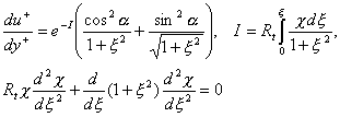
The
boundary conditions are set as follows
(2)
![]()
where
a is the shooting parameter.
Let us suppose that
the velocity profile has a logarithmic asymptotic, i.e.
![]()
Assuming that ![]() we have from the
first equation (1):
we have from the
first equation (1):
![]()
and
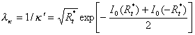
therefore ![]() where
where ![]() . This equation gives the continuous spectrum of the
turbulent scales,
. This equation gives the continuous spectrum of the
turbulent scales, ![]() , as it should be in the real turbulent flow. The
spectrum of this model is related to the spectral characteristics of wall
turbulence.
, as it should be in the real turbulent flow. The
spectrum of this model is related to the spectral characteristics of wall
turbulence.
The function ![]() can be
considered as a spectral density. The inverse length scale versus the Reynolds
number is shown in Figure 1a. This
type of a spectral density is similar to the spectral density of the streamwise
velocity fluctuations in the turbulent boundary layers. The function v0+(Rt)
is shown in Figure 1b. This type of spectrum is similar to the spectral density
of the transversal velocity pulsation. Both functions represent the
constructive model of the hydrodynamic chaos in the constructive theory of
turbulence.
can be
considered as a spectral density. The inverse length scale versus the Reynolds
number is shown in Figure 1a. This
type of a spectral density is similar to the spectral density of the streamwise
velocity fluctuations in the turbulent boundary layers. The function v0+(Rt)
is shown in Figure 1b. This type of spectrum is similar to the spectral density
of the transversal velocity pulsation. Both functions represent the
constructive model of the hydrodynamic chaos in the constructive theory of
turbulence.
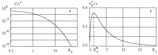
Figure 1: a) The inverse length scale versus the Reynolds number of
dynamic roughness in double logarithmic scale. This type of a spectral density
is similar to the spectral density of the streamwise velocity fluctuations in
the turbulent boundary layers.
b) The normalised turbulent velocity scale versus the Reynolds number of
dynamic roughness. This type of spectrum is similar to the spectral density of
the normal to the wall velocity pulsation [4].
The spectral density of the streamwise velocity pulsation can be defined
as follows
where w is the
characteristic radian frequency, k=w/U is the flow wave number (Taylor's frozen
turbulence hypothesis). To compare the spectral density with experimental data
let us suppose that ![]() ,
Therefore the Reynolds number calculated on the dynamical roughness parameters
depends on the frequency,
,
Therefore the Reynolds number calculated on the dynamical roughness parameters
depends on the frequency,
![]() ,
,
where
A is the parameter, H is the boundary layer height. Therefore the
spectral characteristic of the turbulent flow is related to the eigen spectrum
of the value problem (1-2). In general case it can be the power series
![]() .
.
Practically
we can test one first term of this series. Then the spectral density can be
proposed in the form
(3)
![]()
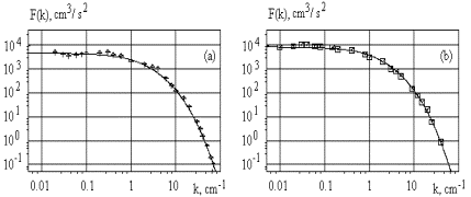
Figure
2. The estimated spectral density of the streamwise velocity pulsation in the
turbulent channel flow (solid lines) for y+=4.9 (a), and y+=11.7(b),
and the experimental data by Hussain & Reynolds.
where cK is the normalising
factor. The spectral density given by equation (3) is shown in Figure 2 (solid
lines) together with the experimental data [3] obtained in the turbulent
channel flow. As it was established both spectral density parameters cK
and A slowly depend on the distance from the wall. The best correlation with the experimental data was found
in the viscose sublayer - see Figure 2.
The
von Karman constant k was calculated recently with the constructive theory of wall turbulence
as follows
This
equation gives k =0.3931 that closed to the experimental quantity obtained by Perry et
al (2001) and Österlund (1999).
To
read more about the constructive theory of turbulence copy ZIP file (261K) with MS Word2000 doc: "Theory and constants of wall
turbulence" by A P Trunev.
References
1.
Trunev A. P. Theory of Turbulence, Russian Academy of
Sciences, Sochi, 1999.
2.
Trunev A. P. Theory of Turbulence and Turbulent Transport in the Atmosphere. WIT
Press, 180 p., 2001.
3. Hussain A. K. M. F. & Reynolds W. C. Measurements in fully
development turbulent channel flow, J.
Fluid Ing. 97, 568-80, 1975.
4. Tennekes H. & Lumley J. L. 1972 A
First Course in Turbulence, MIT Press, Cambridge, Massachusetts.
5.
Perry, A. E., Hafez, S.& Chong, M. S. 2001 A possible reinterpretation of the Princeton superpipe data, J. Fluid Mech., 439, 395-401.
6.
Österlund, J.M. 1999 Experimental studies of zero pressure gradient turbulent boundary layer
flow. Doctoral thesis. Stockholm.