Correlation between extraterrestrial factors and some terrestrial processes: Case Study

Sergey Tarassov, (Canada) tarassov@rogers.com

Alphee Lavoie, (USA) alphee@attbi.com

"In summation, after more than 25 years of research in this field of solar system science, I can say without equivocation that there is very strong evidence that the planets, when in certain predictable arrangements, do cause changes to take place in those solar radiations that control our ionosphere."

John H. Nelson, RCA Communications. Cosmic Patterns. 1974.

Weather prediction is a very complicated process dependent on various factors. Temperature, pressure, magnetic fields, sunspots, and human activity - everything has its part in the process of weather formation. Some of these can be described by corresponding differential equations; others are only an object of scientific observation. The influence of sunspots on life on Earth (including weather) is studied nowadays in different countries. But what about the cosmic neighbors of the Earth – the planets of our solar system and smaller cosmic objects? What if they also have some influence on the weather? Are there any correlations between these extraterrestrials and some processes on the Earth? Planets have some physical parameters that can be calculated, such as, their mass, velocity, parameters of their orbits, distances, etc. We propose some other approach that allows for taking into account any correlations between some weather parameters and some astronomical characteristics of the planets.

We are not alone in this thinking or the first in this field. There has been some research on the subject during past decades in different countries. Worth mentioning are the theoretical attempts of three great Russian thinkers of the Twentieth Century - Vernadsky, Tsiolkovsky and Chizhevsky. We also need to recognize the work of Dr. John Nelson for NASA  (John Nelson, "Short-wave Radio Propagation Correlation with Planetary Positions" RCA Review, March 1951). Dr. Theodore Landscheidt made an overview of his research of solar activity in his books and articles.

We have spent many years trying to answer one simple question: are there any correlations between cosmic factors and different physical processes? If there are, what are they? It took us some years to create instruments for our research. Now we want to apply these instruments, i.e., our software programs, in some areas of our special interest. We have already used these programs in analyzing large data series. We have found that there are correlations between cosmic factors and some processes on the Earth. We have also found that such correlations are non-linear. But to find a correlation is not everything. The most important thing is to use this correlation for modeling and forecasting a real physical process. This article is our attempt to explain our approach to weather forecasting and the forecasting of sunspot activity.

We analyzed the time series for high temperatures in Hartford, Connecticut; data included the period from 1.1.1949 up to 7.31.1998 (18,000 research points). We chose this data only because of their availability. (We are willing to repeat this analysis for any other data set).

First of all, we prepared the data for the analysis. It means that for the research on temperature we take into account the annual trends and work with normalized temperatures.

Then we calculated planetary positions, their velocities, accelerations, distances and angles between planets, and some major asteroids, etc. all within the time interval that is defined by our data set.

The next step is to compare these two data sets in order to find any correlation. We used different modifications of regular statistical methods for this comparison.

And finally - we used the results of the previous step for the forecast. To perform this, we have developed a specialized neural network. This neural network works with a huge amount of data (for example, the specialized neural network for sunspot activity analysis has approximately 5000 inputs; we have used about 50000 points for the learning process). The reason behind using the neural network is in the nature of cosmic factors. We have found that their influence is non-linear (we will not show this in this article though it has been found in stock market analysis). 

It is NOT a 100% forecast and we are not answering all questions about the process analyzed. We only humbly assume that it will help to add some more percentages to the accurate forecast made by various professionals in the field. Our approach is rather universal - it can be used for any data sets. Its purpose is finding correlations of the process analyzed and some cosmic (or extraterrestrial) factors.

One of the methods used for analysis is the Efficiency Test. The idea is very simple. We find the average parameter for: all dates when some cosmic factor occurs, all dates a day before and a day after this event, all dates two days before and two days after the event, all dates three days before and three days after, etc. We then put all these average meanings into a diagram that shows the changes of the parameter analyzed around the date of the cosmic event. It gives us an idea about possible correlations. Here we can make a hypothesis. Then we go back and simply count the number of times when such a hypothesis worked and when it does not. Thus, we arrived at a statistic for our data sample to help us to draw a conclusion about the hypothesis.

What do we do practically? We define the time interval for analysis and look for some cosmic factor within this interval. The "cosmic factor" could be a special position of some planet, some angle between two planets, some special cosmic pattern involving two or more planets or objects (for example, eclipse that involves the Sun, the Moon, the Earth), - anything that takes place in the space and can be described as a single, discreet event. This event occurs at some dates within the interval; it is our sample.  For every single date of this sample, we normalize the parameter analyzed (i.e., temperature) around the date of the event, i.e., we mark the date when the cosmic event occurs as day "0"; we take the high temperature of this day as 0: [T(0)-T(0)=0]. The day before this event will be a day "-1". The high temperature of this day is taken according to the temperature of the day "0": [T(-1)-T(0)]. We do the same for a day after an event (day "1"), for two days before and after (days "-2" and "2"), three days, etc. We have tried even 10 days before and after the event, but the smaller intervals usually show the picture rather well. Then we take all temperatures for all days "0"  and find their average (that is =0, of course); it is a central point of the diagram. After that we take temperatures for all days "1", calculate their average and put it into the diagram. We do the same for all days "2", "3", "4" ..., "-1", "-2", "-3", "-4" ... The results that are shown on a diagram allow us to make a hypothesis about the correlation between this cosmic event and the high daytime temperature.

For example, let us study such event as the change of the direction of planetary motion. Planets, of course, always move in the same direction inside the heliocentric coordinate system.  Change of direction relates to geocentric system of coordinates. Within this system, the Earth is the center, and planets move around on different trajectories. To an observer somewhere on the Earth's surface, planets go in one direction (called direct motion), then move slower until they stop. After that, they go backwards (called retrograde motion), until the next stop. Then they renew their direct motion. We assume that it is worth a try to analyze the process happening on the Earth’s surface within the geocentric system of coordinates, and the important points of planetary trajectory within this system may give us some results.

To be more specific, we define the event researched as Venus becoming direct. The Efficiency Test for this event is shown here (Fig.1):

Fig.1. The Efficiency Test for Venus becoming direct; temperature drops.

This research has been done with the program "Market Trader Expert" developed for financial market analysis, and there are some financial symbols in the windows. We use this program to analyze other data sets, not only financial ones. So please - don't bother with all the prices and dollar signs, all necessary symbols will be explained.

The program has found that within the observed interval, Venus becomes direct 29 times. The temperature change distribution is shown on a histogram in the right part of the window. You can see that the temperature begins to drop 3 days before this event and goes up the next day after that. The temperature drop during 4 days (3 days before the event and a day after) is about 10% (comparing to the temperature of the day "0") and is shown by the blue arrow; it takes place 21 times and does not happen only 8 times.

Another arrow combines days when the temperature goes up after Venus becomes direct; it shows 20 up and 9 down (Fig.2).

Fig.2. The Efficiency Test for Venus becoming direct; temperature goes up.

Here we can make two hypotheses: 1) temperature drops three days before Venus becomes direct and a day after that; 2) temperature goes up the next day after Venus becomes direct. The first hypothesis is true 21 times from 29; the second hypothesis is true 20 times from 29. Looks like these hypotheses work quite well and we can use this hypothesis for weather forecasts. Dates when Venus becomes direct can be easily calculated astronomically, and next time when it will take place we can assume the temperature drops 3 days before the event and the temperature rises the following day. But our example has only 29 dates for analysis; it does not allow for a statistically reliable conclusion. We need to test this hypothesis with more data.

A similar research has been done for all points when Venus becomes retrograde (not shown here). In these cases, the temperature primarily goes up.

Now, let's take another event: Mercury becomes retrograde. The Efficiency Test for this event is shown on Fig.3:

Fig.3. The Efficiency Test for Mercury becoming retrograde.

According to this diagram (Fig.3), we can make a hypothesis: the temperature drops during 4 days after Mercury become retrograde. This event has occurred 146 times within the time interval researched. The hypothesis works 83 times and does not work 63 times out of the 146.

This result can be approved statistically; a chi-squared test of statistical significance (i.e. Pearson test) gives 1.369 amount for 1 degree of freedom and P=0.15. To continue the statistical analysis, we should test the hypothesis that such a correlation exists (i.e., a null hypothesis is that the temperature drops and ups are 50-50; a researched hypothesis is that the temperature goes down whenever Mercury becomes retrograde). We won't do that because of two considerations: 1) we are not sure that random temperature drops are 50% of all temperature changes; 2) we are doubtful that here we are dealing with the normal distribution, so we must use the methods of nonparametric statistics. Also, our research on financial markets shows that the cosmic factor correlations are non-linear. We propose another way: to create a working forecasting model instead of doing time-consuming statistical calculations; the Efficiency Test can be used only as an instrument to find some tendencies or an hypothesis that could (or could not) be true.  

Efficiency Tests for other planetary directions are shown below (Fig.4, 5, 6). Some considerations on statistical results for these examples have been mentioned above.

Fig.4. The Efficiency Test for Jupiter becoming direct.

Here, the temperature goes down 2 days after Jupiter goes direct; it is true 29 times out of 42 (29 down/13 up).

Fig.5. The Efficiency Test for Saturn becoming direct.

The temperature goes up 4 days before Saturn becomes direct and then begins to drop; it is true for 27 times out of 45 (27 down/18 up).

Fig.6. The Efficiency Test for Mars becoming retrograde.

The temperature drops until the 4th day after Mars has become retrograde; it works 15 times out of 23 (15 down/8 up).

We can make the same analysis for any cosmic factor. Let's try now another one that involves position and distance between planets; for example, the 120-degree angle between Jupiter and Uranus (we take the distance as an angle, or the difference of the ecliptic longitudes for the two cosmic objects). Fig.7 shows the Efficiency Test for this event:

Fig.7. The Efficiency Test for 120-degree angle between Jupiter and Uranus.

Within the observed interval, this event happened 13 times. We assume (according to the Efficiency Test) that the temperature goes up two days after this event; the temperature goes up 11 times against just 2 drops. So, next time the angle between Jupiter and Uranus is 120 degrees (astronomers can tell us about that), we should suppose the temperature would go up the same day. (And it will drop 4 days before...). Some considerations on statistical results for this example have been mentioned above.

Above, we have shown results of the Efficiency Tests for just two types of cosmic factors: change of the direction of planetary motion and the angle between planets. For our data sample, some of them have correlations to the temperature change (temperature drops within three days before Venus becomes direct and goes up a day after that; temperature goes up during two days after reaching the exact angle between Jupiter and Uranus at 120 degrees); other correlations are not so obvious (temperature drops when Mercury becomes retrograde).  We can take any cosmic event and check its correlation to temperature changes. But, as we have mentioned above, effect of cosmic factors on physical processes has a non-linear structure. One of the best methods to create a model of a non-linear system is a neural network.

According to Nikola K. Kasabov's book "Foundations of Neural Networks, Fuzzy Systems, and Knowledge Engineering" (The MIT Press, 1998), the neural network is "a biologically inspired computational model which consists of processing elements (called neurons) and connections between them with coefficients (weights) bound to the connections, which constitute the neuronal structure, and training and recall   algorithms attached to the structure. Neural networks are called connectionist models because of the main role of the connections in them." The neural net studies the information about the process researched and adjusts it to the synaptic connections existing between the neurons. It is called the learning process. "Learning typically occurs by example through training, or exposure to a truthed set of input/output data where the training algorithm iteratively adjusts the connection weights (synapses). These connection weights store the knowledge necessary to solve the specific problems" (PNNL, Battelle Memorial Institute Bulletin). 

We have developed our own special neural network (its type is a multi layer perceptron) that uses the astronomical factors as input neurons and gives the normalized temperature as output. But the universal structure of the neural networks allows for adding input other than astronomical factors.

The available data set (high temperature for Connecticut, 18,000 research points) has been divided onto two parts: the learning interval and testing interval. Points from Jan. 1, 1949 to Mar. 7, 1995 are used as a learning interval for the neural net; other points (Mar. 8, 1995 up to Jul. 31, 1998) serve to test these models.

The result is shown on Fig.8:

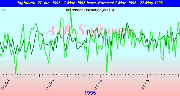
Fig.8.

Here, the light green line is the normalized temperature; the dark green line shows the neural net's forecast. The vertical line for Mar 7 1995 is the bound between the learning interval and forecast. The closer to the bound, the more accurate the forecast is. Both green lines, light and dark, have the same time and ordinate scales; we estimate these lines visually. Here we need to use a correlation coefficient between a real physical process and neural net forecast. But it is not discussed here, because right now we are on the step of model searching; correlation coefficients are the next step.

Fig.9 and Fig.10 show the forecasts for the following dates:

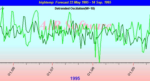
Fig.9.

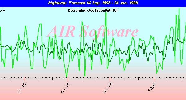
Fig.10.

Further results become chaotic (Fig.11, 12, and 13):

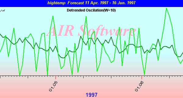
Fig.11.

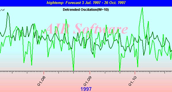
Fig.12.

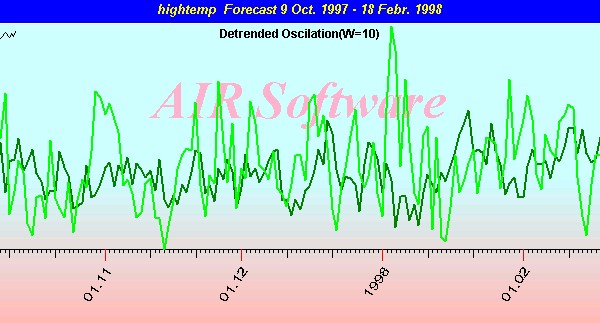
Fig.13.

The farther from the bound, the lesser the accuracy. To make the forecast more accurate, the neural net should be learned on some new sets of data (i.e., we need to move the bound between learning and testing intervals from time to time).

We have some considerations upon the reasons of forecast fading through the time which can be discussed.

Beside the temperature, we have tried to analyze sunspot activity. We have some predecessors in this field:

"In summation, after more than 25 years of research in this field of solar system science, I can say without equivocation that there is very strong evidence that the planets, when in certain predictable arrangements, do cause changes to take place in those solar radiations that control our ionosphere. I have no solid theory to explain what I have observed, but the similarity between an electric generator with its carefully placed magnets and the Sun with its ever-changing planets is intriguing. In the generator, the magnets are fixed and produce a constant electrical current. If we consider that the planets are magnets and the Sun is the armature, we have a considerable similarity to the generator. However, in this case, the magnets are moving. For this reason, the electrical-magnetic stability of the solar system varies widely. This is what one would expect."

- John H. Nelson, RCA Communications. Cosmic Patterns. 1974.

"It is found empirically that solar activity is preceded by planetary conjunctions. A long-range prediction technique has been in use for 2.5 years, which predicts flares and proton events months in advance."

- J.B. Blizzard, Denver University. American Physical Society Bulletin #13, June 1968.

We have done some research on this correlation (planetary conjunctions) for sunspot activity data for the years 1849 - 2002 (August) presented by World Data Center for sunspot index. The data from 1848 to 1996 y.y. were used as a learning interval, other data - as a test of the forecast ability.

We began with the Efficiency Test. Here are some examples (Fig.14 and 15) exposing the correlation between planetary conjunctions and Sunspot activity:

Fig.14. Efficiency Test for Jupiter - Mars conjunction and sunspot activity index.

The Efficiency Test shows that for Jupiter - Mars conjunction (in heliocentric system) the sunspot activity index goes down 4 days before the conjunction and begins to rise at the day of the event. Within the interval observed, it has happen 43 times of 63 tries; it was not true 20 times. Some considerations on statistical results for this example have been mentioned above.

Fig.15. Efficiency Test for Jupiter - Mercury conjunction and Sunspot activity index.

Jupiter - Mercury conjunction (in heliocentric system) takes place more often than Jupiter - Mars. So here we have 625 points for analysis. The sunspot activity index goes down 4 days before the exact conjunction; it continues to go down two more days after, and during these two days the drop is bigger. So hypothesis in this case sounds as "The sunspot activity index goes down two days after the exact conjunction between Jupiter and Mercury takes place". This hypothesis works 380 times and does not work 245 times within the interval observed. This result is statistically approved. We tested it with null hypothesis. We could not choose a null hypothesis as "The sunspot activity index equally goes up and down" - because a simple observation of the diagram of this index shows equal change of the index, not amount of ups and downs. This index goes up fast (like receives some impulse) and then goes down slower. So we could not take the null hypothesis as 50% ups and downs. We did it this way: we chose 625 random points and created the Efficiency Test for this random data. Then we repeated this process for 625 other random points, five more times. Standard statistic methods for this random data show the average amounts of downs and ups as 340.6 and 284.4. It allows us to do the Pearson test for statistical significance and gives a chi-square amount as 4.5 and p=0.04; it means that the hypothesis about the sunspot activity index drop at the Jupiter - Mercury conjunction with a reliability of 96%. (If we take into account the dispersion of the Efficiency Test results, we have the reliability of this hypothesis 70% through 96%.)

If we take the opposition of Jupiter - Mercury, the Efficiency Test will show the rise of the sunspot activity index (Fig.16):

Fig.16. Efficiency Test for Jupiter - Mercury opposition and sunspot activity index.

Planets can form other angles between them, not a conjunction alone; some of these angles have a correlation to the sunspot activity index. We can continue to do the Efficiency Test for every possible angle between every possible pair of planets, or we can use another technique that is called “Composite." The idea behind these methods is to represent the data of the sunspot activity index in angular coordinates; then we look for a relationship between the sunspot activity index and the angle of some pair of planets. The composite for angle between Jupiter and Saturn (Fig.17) yields quite interesting results:

Fig.17. Composite for sunspot activity index as a function of the angle between Jupiter and Saturn.

The upper diagram shows how the sunspot activity index depends on the angle between Jupiter and Saturn (heliocentric system).

But again - all the above results must be tested for statistical reliability. Or we can use them all as a hypothesis that will be used as input for the neural network. The neural network for the sunspot activity index forecast gives us such results (Fig.18):

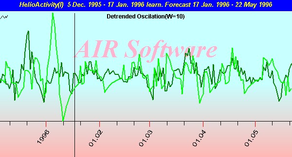
Fig.18. Neural net model for sunspot activity index.

Here, the diagram represents a normalized sunspot activity index (the light green line) and its forecast by the neural net (the dark green line). The vertical line is a border between learning and forecasting intervals; the neural net forecast can be seen after this border. The target function used here is (I - IMA10)/IMA500, where I stands for the Sunspot Index, and IMA10 and IMA500 stand for the moving average of the index within 10-days and 500-days intervals accordingly. We tried to receive the short-term forecast. In this case, the neural net uses heliocentric planetary angles as input.

Figs.18 and 19 through 22 show the results for different models and different neural net analysis for the sunspot activity index (the learning bound is May 26, 1995). These pictures illustrate our work in process.

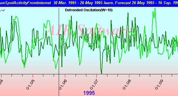
Fig. 19. Another neural net model for sunspot activity index (continued on Fig. 19 - 21).

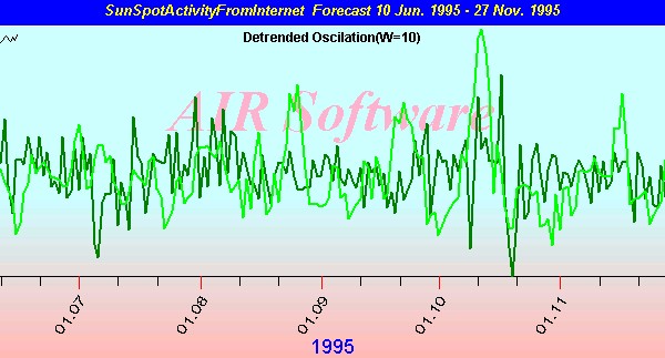
Fig. 20. Neural net model for sunspot activity index

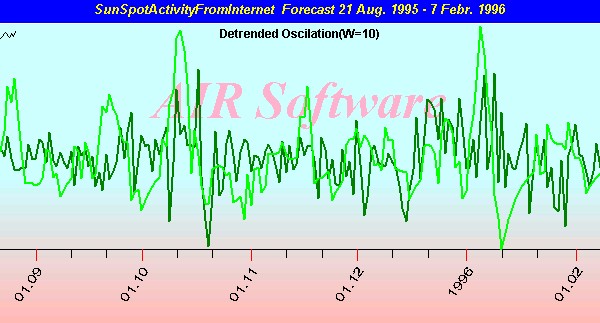
Fig. 21. Neural net model for sunspot activity index

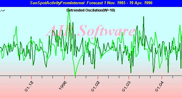
Fig. 22. Neural net model for sunspot activity index

As we have mentioned above, the nature of the impact of cosmic factors to the physical process is non-linear. A single factor (i.e., the angle between Mars and Venus) does not influence the same way all the time. It looks as if these single factors act as a complex. It means that the number of hidden neurons of the neural net is rather large and such a neural net takes a lot of time for learning. Now, we try to understand the following: a) what cosmic factors are more important for modeling a specific physical process (the standard techniques of finding the most significant factors like "boxing counting" cannot be used because of huge volume of input); b) how these factors should be formalized when they are used as neural network inputs (we use now Fuzzy NN mostly); c) what is the optimal structure of this neural network (number of neurons at the hidden layers and type of activation function). We continue our research on the subject. Solving the problem takes time because we try different models and hypothesis as variable inputs for the neural net. But even now we can be sure that the neural net exactly models the process of geomagnetic activity (or other physical processes - in other cases).

We created our neural net as an open system. It means that we can analyze any time series of data and use as input any parameters (not only astronomical) that are related to the process researched.

Correlations between extraterrestrial factors and physical processes on the Earth are reality nowadays. Methods described in this article allow investigating them. As it was mentioned above, we are not creating new physical models or theories for some real processes. It is a task for others. To our mind, one of the possible ways to explain how these correlations work is in minor variations of the gravity potential. It fits to the modern scientific paradigm (especially non-linear dynamics) and appeals to non-equilibrium processes at atmosphere boundary layers. But this is a theme for future discussion. 

Besides, the neural net we have created works now as a black box: it takes data and finds the connection weights. We see results, but we don’t know exactly how every parameter works. There are some ways to extract the knowledge from the neural net; we work on it also trying to make this “black box” at least “a grey one”.